Disturbance mapping
Workflow: Mapping disturbances
We organized the mapping workflow into six broad steps, starting from defining an area of interest to creating up-to-date disturbance and validating it. Not all the steps may need to be completed if, for example, there were no gaps in the coverage of disturbances. Likewise, the workflow is flexible and does not necessarily need to be completed sequentially. In this particular workflow we’ve assumed that the end goal is to create an up-to-date anthropogenic disturbance map for a user-defined study area.
Finally, we note that, although important, this workflow does not incorporate machine learning algorithms for automated classification of disturbances. It is meant to be applied by anyone with access to a computer and the internet and does not require any special GIS, remote sensing, or data analysis skills. The workflow has been tested and refined using project areas in the Yukon and British Columbia. It will continue to be revised iteratively through experience and user feedback.
The flowchart below provides an overview of the disturbance mapping workflow and its six steps. Each step is then described in more detail in the following paragraphs.
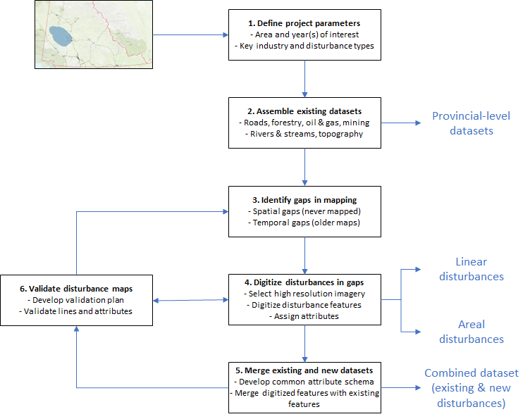
Figure 1. Flowchart outlining the six broad steps used to develop an anthropogenic disturbance map for a study area of interest.
Step 1. Define area and disturbances of interest
The first step of a new mapping project is to define the area of interest, the year(s) of interest, and the key anthropogenic disturbance types of interest. The area of interest (AOI) can either be an existing polygon or a user-defined polygon. Examples of existing polygons in Canada include watersheds (e.g., fundamental drainage areas or FDAs), ecoregions, or caribou ranges. Alternatively, a user-defined polygon can be digitized using QGIS. The selected polygon should then be saved as a layer in a geopackage format (“.gpkg”). At this point it is also important to consider the coordinate reference system (CRS) that will be used as well as the resolution of any raster data that will be used, including satellite imagery. The intitial geopackage should thus include the AOI boundary layer in the CRS that will be used for the project.
Another important consideration is to identify the year(s) of interest for the project. If the objective of the project is to create a disturbance map for the current time period, this will limit the search of data sources to the most recent datasets available. Since it is unlikely that all available data sources are current, this will also require a search of recent, cloud free, satellite imagery (see Step 3). A combination of existing thematic maps and recent satellite imagery will thus often be necessary to create a temporally homogeneous coverage of the AOI. In some cases, the objective might be to look at change over time, requiring two or more time periods, and consequently the search for historical data source. The choice of historical time periods to map will depend on available data sources, including older imagery and aerial photos and objectives of the project.
The third consideration in step one is to identify which anthropogenic industry and disturbance types will be mapped. The most common approach is to include all linear and areal disturbances that are detectable at a set scale, usually limited by the availability of satellite imagery for the AOI and year desired. In other cases, interest might be focused on the one industry, for example to evaluate the effects of mining on wolverine occupancy. Anthropogenic disturbance types to be mapped can be identified through local knowledge, a literature review, or expert consultation. In the boreal region, many disturbances are related to, but not limited, to mining, forest management, and oil and gas activities. The key task here is to use, adapt, or develop a (hierarchical) classification scheme to organize disturbance types into broader categories and subcategories. Such a scheme will facilitate the systematic classification of disturbances using remote sensing data. A possibility is to adopt or adapt an existing classification scheme for disturbances. For example, in the case study below, we use the classification system developed by the Yukon Government for surface disturbance mapping (Government of Yukon 2022). Alternatively, a global hierarchical framework classifying disturbances can be used (IUCN?).
Products for this step include:
- A GeoPackage file (https://www.geopackage.org/) with a vector layer of the area of interest (AOI) in the coordinate reference system (CRS; https://en.wikipedia.org/wiki/Spatial_reference_system) to be use throughout the project.
- A spreadsheet describing the industry and disturbance types that will be the focus of the mapping project.
Step 2. Assemble existing datasets
The main objective of this step is to compile existing datasets related to anthropogenic disturbances from various sources, including governmental agencies, research institutions, and remote sensing repositories. The datasets should encompass a wide range of disturbance types, such as linear infrastructure, forest harvesting, mining activities, and energy development. Examples include roads, cutblocks, seismic lines, and open pit mines. Additionally, ancillary data sources such as topography and hydrology should be considered as they can often be used to enhance interpretability. In some cases, some disturbance types may have more than one source of data. For example, in most provinces forest resources inventory data is collected regularly and made available publicly. The data vary greatly by province or territory in terms of attributes collected and year(s) of inventory. Complementary to this data source is a time series harvested areas based on 30-m Landsat imagery for the years 1984-2019. In many cases, both sources may need to be used to create a seamless and current map of harvest areas for an AOI. Table 2 provides several lists of datasets that can be used as a starting point for projects based in Canada.
Once datasets have been compiled, they will need to be processed to create a comprehensive database for the project using a consistent coordinate reference system (CRS). Each selected dataset should be clipped to the AOI and reprojected to the project CRS. Sample scripts to do this are provided on the accompanying GitHub repository and illustrated in the case studies.
Products for this step include:
- A “metadata” table that describes each dataset that will be considered for use in the project. For each datasets, the table should include information on geographic coverage, year, resolution, input data sources, download URL or contact, date of acquisition etc.
- A “gisdata” folder that contains all orginal datasets that were acquired and that will potentially be used in the mapping project.
- A GeoPackage (see Step 2) that comprises all clipped and reprojected datasets that will be used in the next steps, along with any code and documentation to enable replication.
Table 2. Existing data sources for Yukon, BC, Alberta, and NWT. Each list is regularly updated.
| Dataset | Location of annotated list |
|---|---|
| Yukon | https://github.com/beaconsproject/disturbance_mapping/blob/master/docs/data_yt.csv |
| BC | https://github.com/beaconsproject/disturbance_mapping/blob/master/docs/data_bc.csv |
| Alberta | https://github.com/beaconsproject/disturbance_mapping/blob/master/docs/data_ab.csv |
| NWT | https://github.com/beaconsproject/disturbance_mapping/blob/master/docs/data_nt.csv |
| Canada | https://github.com/beaconsproject/disturbance_mapping/blob/master/docs/data_national.csv |
| Global | https://github.com/beaconsproject/disturbance_mapping/blob/master/docs/data_global.csv |
| Web services | https://github.com/beaconsproject/disturbance_mapping/blob/master/docs/web_services.csv |
| Satellite imagery | https://github.com/beaconsproject/disturbance_mapping/blob/master/docs/remote_sensing.md |
Step 3. Identify spatial and temporal gaps in coverage
Once all essential existing datasets have been assembled into a GeoPackage file, the next step is to identify if and where spatial and temporal gaps in coverage exists. This step is important because it will identify and limit where new data needs to be acquired through digitization as described in Step 4. There are several possibilities. In some cases, disturbance datasets will cover the entire AOI for a specific disturbance type e.g., railroads and cutblocks. In other cases, an attempt to map all disturbance types may have been made for a subset of the AOI. In such cases, the data may be accompanied by an “extent of mapping” polygon indicating the spatial boundaries of the mapping project. In the best case, the year of mapping and/or data sources used would also be included. This is the case with the Yukon Government surface disturbance mapping initiatives, which will be described further in the case study. If that information is not available, the user will need to compare various data sources (thematic and imagery) to attempt to determine the year for which the information is valid.
The key task here is to review the database thoroughly to identify any areas where there are gaps in the coverage. Each disturbance layer in the GeoPackage should be reviewed separately and/or together to evaluate its completeness for each identified disturbance type. Gaps can then be recorded using a spatial grid, for example a 10km x 10km grid intersecting the study area. The case study will provide an example of this. This will allow for a quick view of grid squares that will need to be filled through digitizing. Temporal gaps also need to be identified by looking for attributes with information about the year of mapping or underlying data sources used to generate specific datasets. If the year of the data is significantly different from the target year, this should be identified as a temporal gap due to the age of the information. Likewise, if there is no attribute information, this should also be identified as a gap due to lack of information. Information on temporal gaps can also be added to the gap grid.
Products for this step include:
- A grid map and accompanying table describing spatial and temporal coverage in coverage. The specific disturbance types that are missing should also be indicated in the table. This grid map and table will be used to assess whether gaps can be filled with detailed disturbance mapping using recent high resolution satellite imagery.
Step 4. Fill gaps through satellite imagery digitization
The objective of Step 4 is to fill any spatial or temporal gaps in the AOI that were identified in the previous step. To fill these gaps, we adapted a methodology for digitizing surface disturbance data from satellite imagery based largely on an approach developed by the Yukon Government (YG 2023). The approach is based on manual digitization of disturbances from high resolution satellite imagery using geographic information system (GIS) software and ancillary data. This step can be divided into four tasks: i) preparation of a data package, ii) selection of appropriate satellite imagery, iii) digitizing linear and disturbance features from satellite imagery (including assigning attributes and confidence level), and iv) ensuring quality control on an ongoing basis.
The project data package should consist of several data layers, including existing anthropogenic disturbances, reference layers (i.e., boundary and grids to guide digitizing), digitizing templates for linear and areal disturbances, and supporting ancillary layers (e.g., rivers and streams). A description of the template layers for linear and areal disturbances and how to create them is provided in the BEACONs Disturbance Mapping Procedures manual. This includes adding several key fields for recording information of industry and disturbance type, year and source of satellite imagery, etc.
The data package should also include the selected satellite imagery downloaded as geotiff files or added as web services within QGIS. Table 3 provides examples of sources of commonly available satellite imagery. Some sources, such as SPOT imagery, are generally not freely available to individuals but may be accessible through partner organizations or government or university agreements. For example, GeoYukon provides complete (mostly cloud free) coverage of the Yukon using SPOT imagery (circa 2021) which is freely available as a web services. An example data package is provided in the case study. Other appropriate satellite imagery sources should be selected based on their spatial resolution, temporal frequency, and spectral bands that are best suited for capturing the disturbances of interest. For example, Landsat or Sentinel may be suitable for mapping harvested areas or wilfires but may not be of high enough resolution to capture seismic lines. If necessary, satellite imagery may undergo pre-processing to enhance interpretability. This includes radiometric and atmospheric correction, image calibration to minimize sensor artifacts, and cloud masking and image mosaicking to ensure data quality. Such procedures are beyond the scope of this paper and our focus is on analysis ready imagery. In the case studies, we illustrate the process of digitizing disturbance features from SPOT imagery. We also note that there is an increasing number of apps that can be used to automate the mapping of disturbances using the Landsat and Sentinel archives on GEE1 (LandTrendr1, Kennedy et al. 2021; BAP2, White et al. 2014). These may be useful for mapping certain types of disturbances over time e.g., see, for example, https://opendata.nfis.org/mapserver/nfis-change_eng.html.
Table 3. Sources of freely available high resolution satellite imagery suitable for mapping anthropogenic surface disturbances at 1:5,000 scale.
| Source | Spatial resolution | Temporal resolution | Example availability |
|---|---|---|---|
| SPOT | 1.5m | GeoYukon | |
| Sentinel | 10m | Copernicus | |
| Landsat | 30m | 1984-2023 | Google Earth Engine |
| ESRI | varies | varies | ArcGIS, QGIS web services |
| varies | varies | ArcGIS, QGIS web services |
1 https://emapr.github.io/LT-GEE/
2 https://github.com/saveriofrancini/bap
Step 5. Merge existing and new datasets
The main objective of Step 5 is to combine the newly digitized linear and areal disturbance features with the existing disturbance featues that were assembled in Step 2. Key to this step is the use of a common attribute schema to facilitate the integration of different sources of data. A common attribute schema should not only include common attributes but a range of acceptable values for all attributes, whether continuous or categorical. Once digitizing is complete and has been reviewed (Step 6) by at least one other project member, the new and existing data can be merged manually using either QGIS or programatically using R. The advantage of using R for this step is that it insures replicability and allows one to add some validation code to check for valid attribute names and values. Sample code is provided on the GitHub repository and illustrated in the Case Studies. Note that this step also assumes that existing features that were found to be no longer visible or in error have been removed or revised prior to merging (see Digitizing manual).
Step 6. Validate and revise maps
The focus of Step 6 is to validate the newly digitized anthropogenic disturbance features and revise the maps if needed. This can be done in one of three ways, with increasing rigour: i) ongoing review of digitizing work by another person, ii) remote-based validation, and iii) field-based validation. In first approach, a second person from the project team (e.g., a supervisor or alternative digitizer) should review and check a sample of the newly digitized features (or all features in more intact areas), preferably on an ongoing basis. In this way, the quality of digitized data can be ensured through multiple rounds of verification and validation.
In the second approach, the newly digitized features are validated using imagery that are of a higher resolution that the imagery that was used to digitize the features. This can include very high resolution (VHR) imagery (e.g., ESRI or Google imagery) or even recent or historical areal photos if available. The selected ground truth data can then be used to assess the accuracy of the mapped disturbances. To do this, the mapped disturbances should be compared with the “ground truth” data to measure discrepancies and identify areas of agreement. The validation results can be used to inform iterative refinements of the workflow, such as selecting additional sources of satellite imagery or auxilliary data, or planning additional validation steps.
In the third and most rigorous approach, independent field-based data is collected and compared to the mapped features. Field-based data can be collected by visiting features in situ either in person (e.g., walking, biking, using quads) or using drones from locations near the features of interest. In addition, field-based validation could include workshops with community members or land users to get their input on local trails and roads. Confirming attributes of mapped features, adding trails that cannot be mapped from satellite imagery, for example snow mobile trails that are only used in the winter. Field-based validation is generally more cost and labour intensive than the first two methods and are not always conducted by agencies charged with disturbance mapping (e.g., ABMI). The design and collection of field-based data is beyond the scope of this paper.
Products for this step include:
- A list of newly digitized lines and polygons and their attributes that were checked by another qualified project member.
- Summary statistics from comparing the newly digitized linear and areal features to higher resolution data from the same time period.