Create builder polygons

Intro

This script generates potential benchmarks, as well as upstream and downstream polygons based on the BUILDER output.

The first step is to locate catchments layer and specify the directory where BUILDER output were saved.

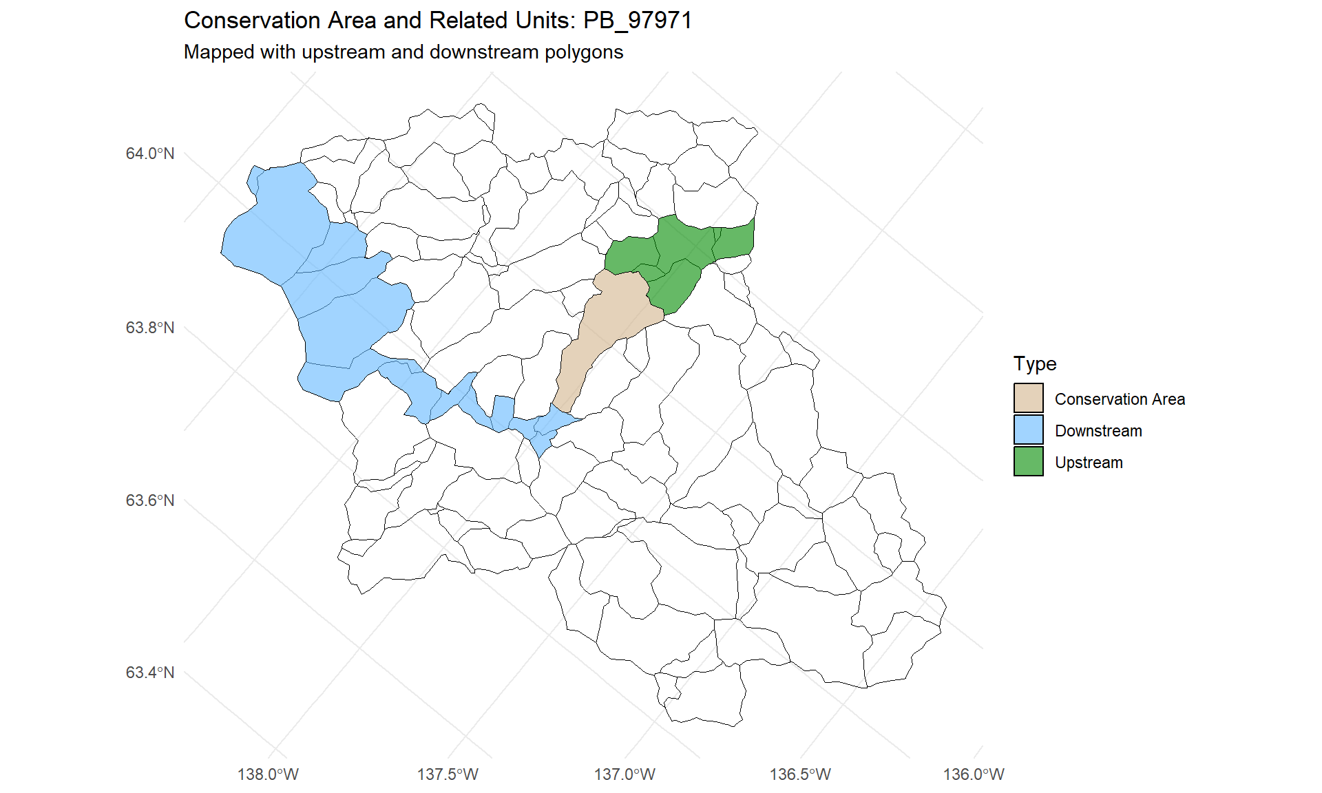
These polygons are then used to assess dendritic connectivity by clipping the stream network to each polygon and analyzing how water flows within its boundaries.

Generate potential benchmarks, upstream and downstream polygons from catchments using BUILDER output files

Function fetch_builder_output allow to read Builder output tables that uses column format. The output can then be passed to dissolve_catchment_from_table to generate polygons using enumerated ‘CATCHNUM’. fetch_builder_output needs the following:

• out_dir: Point to a directory that contains Builder output
• type: Indicate which file to read. Type can be ‘BENCHMARKS’, ‘UPSTREAM’ or ‘DOWNSTREAM’. Default is ‘BENCHMARKS’.

# Load required libraries
library(sf)
library(dplyr)
library(tidyr)
library(utils)
library(ggplot2)
library(RColorBrewer)
library(here)

# --------------------------------------
# SET PARAMS  --------------------
# --------------------------------------
# Set working directory
dirpath <- here(".")

# Source BEACONs functions
source(file.path(dirpath,"R/spatial.R"))
source(file.path(dirpath,"R/builder.R"))
source(file.path(dirpath,"R/utils.R"))

# Folder path to the benchmarkbuilder executable
builder_path <- here("builder")

# Set Builder output path (create the folder structure if missing)
builder_dir <- file.path(dirpath, "output/Builder_output")
if (!dir.exists(builder_dir)) {
  dir.create(builder_dir)
}

# Create the folder structure to receive output polygons
out_dir <- file.path(dirpath, "output/shp_output")
if (!dir.exists(out_dir)) {
  dir.create(out_dir, recursive = TRUE)
}

# Prefix given to identify unique conservation areas
colName <- "PB"


# --------------------------------------
#--RUN
# --------------------------------------

# Use conservation areas as reserve seeds
catchments <- st_read(file.path(dirpath,"data/catchments_sample.shp"))

Reading layer `catchments_sample' from data source 
  `E:\MelinaStuff\BEACONs\git\R_tools_public\data\catchments_sample.shp' 
  using driver `ESRI Shapefile'
Simple feature collection with 108 features and 15 fields
Geometry type: POLYGON
Dimension:     XY
Bounding box:  xmin: -2073549 ymin: 752749.6 xmax: -1946333 ymax: 861999.6
Projected CRS: NAD_1983_Albers

conservation_areas <- st_read(file.path(dirpath,"data/reserves_sample.shp"))

Reading layer `reserves_sample' from data source 
  `E:\MelinaStuff\BEACONs\git\R_tools_public\data\reserves_sample.shp' 
  using driver `ESRI Shapefile'
Simple feature collection with 3 features and 2 fields
Geometry type: POLYGON
Dimension:     XY
Bounding box:  xmin: -2063049 ymin: 815481.9 xmax: -1987393 ymax: 861999.6
Projected CRS: NAD_1983_Albers

# Run BUILDER
nghbrs <- neighbours(catchments)
seed <- seeds(catchments, areatarget_value = 100000000)
builder(catchments_sf = catchments, data_source = "catchment", seeds = seed, neighbours = nghbrs, out_dir = builder_dir, builder_local_path = builder_path, catchment_level_intactness = 0.8, conservation_area_intactness = 1, output_upstream = TRUE, output_downstream = TRUE)

# A tibble: 4 x 44
  PB_94784 PB_95575 PB_95583 PB_95840 PB_95876 PB_95898 PB_95949 PB_96020
     <int>    <int>    <int>    <int>    <int>    <int>    <int>    <int>
1    94784    95575    95583    95840    95876    95898    95949    96020
2    94837    95831    95831    95831    96075    95629    95840    95949
3       NA       NA    95575       NA    97226       NA    95831    95840
4       NA       NA       NA       NA       NA       NA       NA       NA
# i 36 more variables: PB_96075 <int>, PB_97226 <int>, PB_97345 <int>,
#   PB_97440 <int>, PB_97971 <int>, PB_98263 <int>, PB_98271 <int>,
#   PB_98487 <int>, PB_98559 <int>, PB_98569 <int>, PB_98723 <int>,
#   PB_98912 <int>, PB_98960 <int>, PB_99037 <int>, PB_99170 <int>,
#   PB_99304 <int>, PB_99401 <int>, PB_99409 <int>, PB_99418 <int>,
#   PB_99428 <int>, PB_99923 <int>, PB_99941 <int>, PB_100028 <int>,
#   PB_100140 <int>, PB_100688 <int>, PB_100869 <int>, PB_100969 <int>, ...

#############################################
#  Generate potential conservation areas polygons
#############################################
type <- "BENCHMARKS"
out_tab <- fetch_builder_output(builder_dir, type = type)

# Convert builder output tables to polygons
PBx_sf <- dissolve_catchments_from_table(catchments_sf = catchments, 
                                             input_table = out_tab, 
                                             out_feature_id = colName)


#############################################
#  Generate upstream polygons
#############################################
type <- "UPSTREAM"
out_tab <- fetch_builder_output(builder_dir, type = type)

# Convert builder output tables to polygons
upPBx_sf <- dissolve_catchments_from_table(catchments_sf = catchments, 
                                             input_table = out_tab, 
                                             out_feature_id = colName)


#############################################
#  Generate downstream polygons
#############################################
type <- "DOWNSTREAM"
out_tab <- fetch_builder_output(builder_dir, type = type)

# Convert builder output tables to polygons
downPBx_sf <- dissolve_catchments_from_table(catchments_sf = catchments, 
                                             input_table = out_tab, 
                                             out_feature_id = colName)


# Map example
# Get the first conservation area ID
first_pb_id <- PBx_sf$PB[13]

# Filter all layers for this conservation area
pb1      <- PBx_sf[PBx_sf$PB == first_pb_id, ] %>% mutate(type = "Conservation Area")
up_pb1   <- upPBx_sf[upPBx_sf$PB == first_pb_id, ] %>% mutate(type = "Upstream")
down_pb1 <- downPBx_sf[downPBx_sf$PB == first_pb_id, ] %>% mutate(type = "Downstream")

# Combine layers 
overlay_data <- rbind(pb1, up_pb1, down_pb1)

# Plot all layers together
ggplot() +
  geom_sf(data = catchments, fill = NA, color = "black", size = 0.2) +
  geom_sf(data = overlay_data, aes(fill = type), color = "black", alpha = 0.6) +
  scale_fill_manual(
    name = "Type",
    values = c(
      "Conservation Area" = "tan",
      "Upstream" = "green4",
      "Downstream" = "steelblue1"
    )
  ) +
  labs(
    title = paste("Conservation Area and Related Units:", first_pb_id),
    subtitle = "Mapped with upstream and downstream polygons",
    x = NULL, y = NULL
  ) +
  theme_minimal() +
  theme(legend.position = "right")

# Save 
write_sf(PBx_sf, dsn =file.path(out_dir, "CAs_poly.shp"), append = FALSE)
write_sf(upPBx_sf, dsn =file.path(out_dir, "upstream_poly.shp"), append = FALSE)
write_sf(downPBx_sf, dsn =file.path(out_dir, "downstream_poly.shp"), append = FALSE)