BEACONs Representation R Functions

`evaluate_criteria_using_clip()`

The evaluate_criteria_using_clip() function evaluates the specified criteria by clipping them to either individual conservation areas or a conservation network. The evaluation calculates the proportion of each class within the area. If a unique identifier (CAs_id) is provided, proportions are computed separately for each corresponding polygon.

Usage

evaluate_criteria_using_clip(
  conservation_area_sf, 
  criteria_raster, 
  conservation_area_id = NULL, 
  class_values = c(), 
  target_size = NULL
)

Arguments

CAs_sf: sf object of conservation areas.
criteria_raster: Raster object of the representation layer classified into categorical classes
CAs_id: Column in CAs_sf specify unique identifier.
class_values: A vector of classes in representation_raster to generate targets for. Defaults to all classes in the representation_raster.
target_size: The area in km2 that targets will sum to. Default is NULL

📤 Output

A tibble with columns: - conservation_area_id (if provided) - class_value: the list of class_values} - area_km2: the area of each class_value in the CAs_sf} - class_proportion: area_km2/sum(area_km2)} - target_km2

Examples

Running the examples

Download and unzip BEACONs R Tools
Run the examples below.

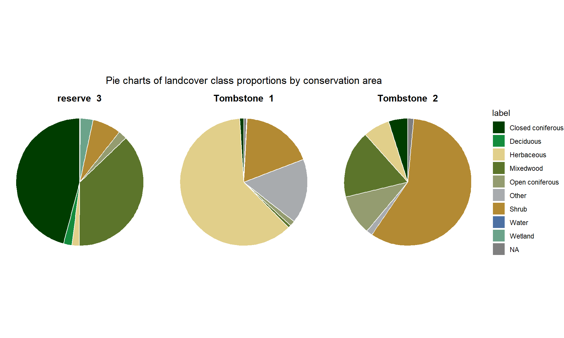
# Load libraries
library(sf)
library(terra)
library(dplyr)
library(here)

# --------------------------------------
# SET PARAMS  --------------------
# --------------------------------------
# Set working directory
dirpath <- here(".")

setwd(dirpath)
source("./R/representation.R")

#Set access path 
reserves_sf <- st_read(file.path(dirpath, "data/reserves_sample.shp"), quiet = TRUE)
nalc <- rast(file.path(dirpath, "data/nalc_sample.tif"))

result <- evaluate_criteria_using_clip(reserves_sf, nalc, conservation_area_id = "reserve")

# ── To display landcover classes proportion per conservation areas ------------
library(readr)
library(ggplot2)

# Read landcover color palette from files
landcover_colors <- read_csv(file.path(dirpath, "data/lc_cols.csv"))

# Join hex code to results
results <- result %>%
  mutate(class_value = as.integer(class_value)) %>%
  left_join(landcover_colors, by = "class_value")

# set number of piechart based on number of conservation areas.
n_chart <- length(unique(reserves_sf$reserve))

# Plot proportion
ggplot(results,
       aes(x = "", y = class_proportion, fill = label)) +  # use label for legend
  geom_col(width = 1, colour = "white") +
  coord_polar(theta = "y") +
  facet_wrap(~ reserve) +
  scale_fill_manual(values = setNames(results$hex, results$label)) +
  labs(title = "Pie charts of landcover class proportions by conservation area") +
  theme_void() +
  theme(strip.text = element_text(size = 12, face = "bold"),
        plot.title = element_text(hjust = 0.5, margin = margin(b = 10))
        )